This vignette will introduce you to partitions().
partitions() provides an alternative approach to
implementing case definitions. In summary, it uses specific temporal
boundaries as the window of occurrence. This differs from
episodes() where the boundaries are calculated as durations
relative to index events. partitions() produces a similar
S4 class identifier (pane) referred to as
panes and share similar arguments with episodes().
To demonstrate this difference, let’s review the homes
dataset below. It has data on household members including their ages.
We’ll attempt to apply a case definition to identify a three-generation
home, where each generation includes individuals aged not more than 16
years apart.
homes <- data.frame(member = c("son_1", "son_2", "daughter_1",
                               "father", "mother", "grand_father", "grand_mother"),
                    age = c(4, 6, 17, 43, 40, 74, 69))
homes
#>         member age
#> 1        son_1   4
#> 2        son_2   6
#> 3   daughter_1  17
#> 4       father  43
#> 5       mother  40
#> 6 grand_father  74
#> 7 grand_mother  69
The simplest approach would be to specify the age bands for each generation. In this context, these are the temporal boundaries.
age_bands <- seq(0, 69, by =17)
age_bands <- number_line(age_bands, age_bands + 16)
age_bands
#> [1] "0 -> 16"  "17 -> 33" "34 -> 50" "51 -> 67" "68 -> 84"

homes$grp_1 <- partitions(homes$age, window = list(age_bands), separate = TRUE)
homes
#>         member age     grp_1
#> 1        son_1   4 PN.08 (I)
#> 2        son_2   6 PN.08 (D)
#> 3   daughter_1  17 PN.09 (I)
#> 4       father  43 PN.10 (D)
#> 5       mother  40 PN.10 (I)
#> 6 grand_father  74 PN.12 (D)
#> 7 grand_mother  69 PN.12 (I)

schema(homes$grp_1, seed = 4,
       custom_label = paste0(homes$member, " \n(", homes$age, " yrs)"))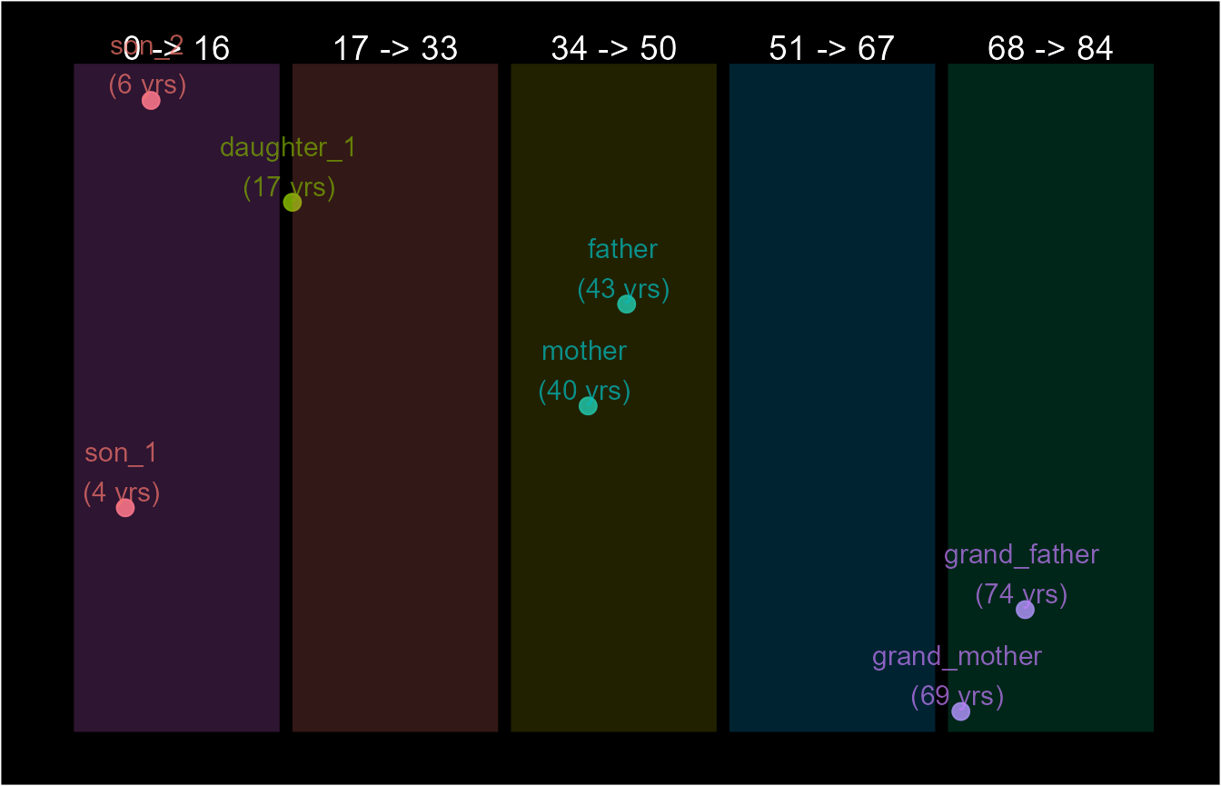
However, we can make the case that the children are all part of the
same generation since no two are older than 16 years apart. This
presents the main difference between partitions() and
episodes(). Unlike episodes(), the duration
(age gaps) between records is not a factor. Here records or events are
linked together simply because they exist within the same interval (age
gap).
To correct this, we can start the age band from age 6 but this
becomes difficult to manage when analysing multiple homes. Instead, we
can use the by or lenght.out argument to
create windows (window) relative to the first event (or
custom_sort) only. Although this makes it more like
episodes(), it is still different since all age gaps are
relative to only one reference event (I).
homes$grp_2 <- partitions(homes$age, by = 16, separate = TRUE)
schema(homes$grp_2, seed = 4,
       custom_label = paste0(homes$member, " \n(", homes$age, " yrs)"))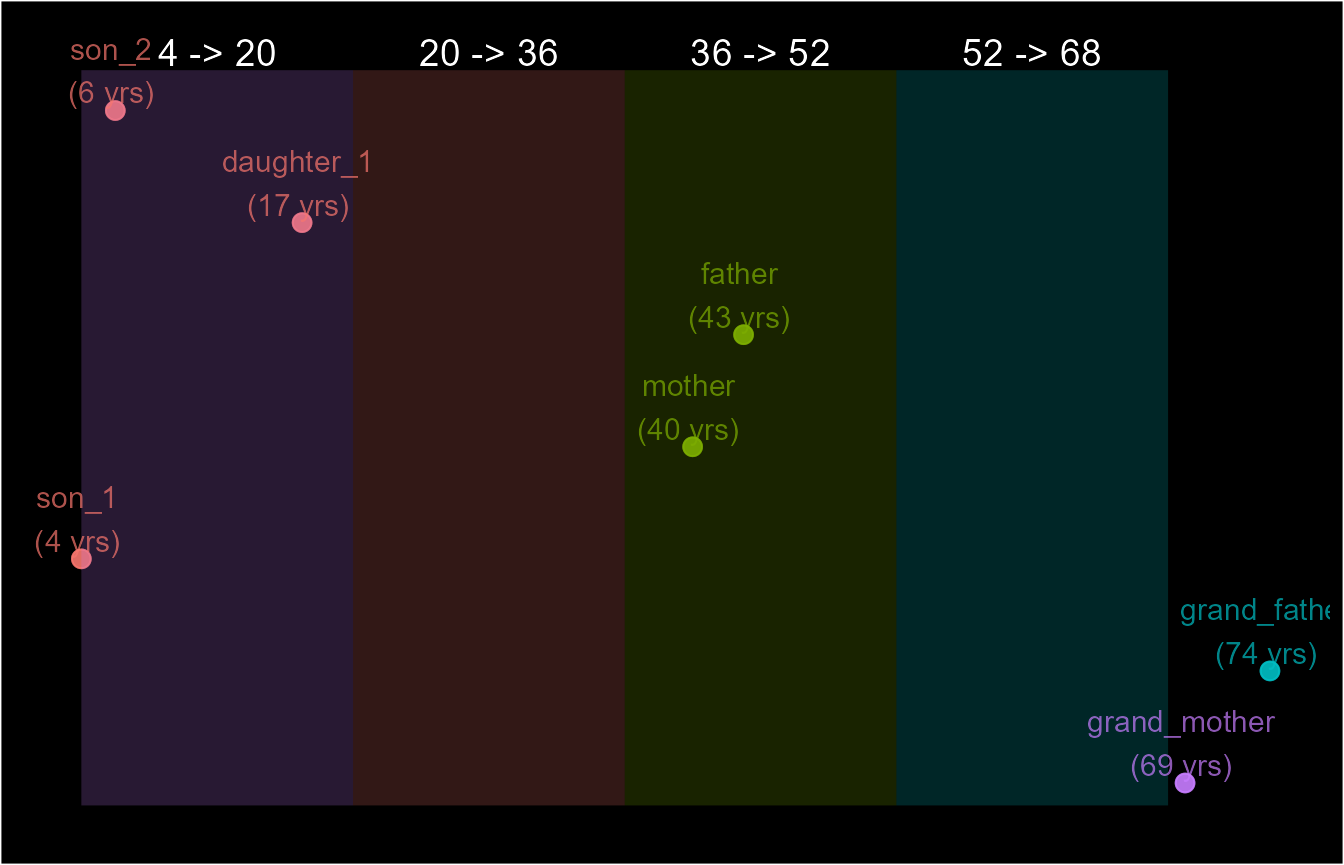
Now that we have identified the generations, we can build on this by linking every record on the conditions that there’s a specified number of generations (windows). Below we ask for three to four generations.
homes$grp_3 <- partitions(homes$age, by = 16,
                          separate = FALSE,
                          windows_total = number_line(3, 4))
homes
#>         member age     grp_1     grp_2    grp_3
#> 1        son_1   4 PN.08 (I) PN.08 (I) PN.1 (I)
#> 2        son_2   6 PN.08 (D) PN.08 (D) PN.2 (I)
#> 3   daughter_1  17 PN.09 (I) PN.08 (D) PN.3 (I)
#> 4       father  43 PN.10 (D) PN.10 (D) PN.4 (I)
#> 5       mother  40 PN.10 (I) PN.10 (I) PN.5 (I)
#> 6 grand_father  74 PN.12 (D) PN.06 (I) PN.6 (I)
#> 7 grand_mother  69 PN.12 (I) PN.07 (I) PN.7 (I)

schema(homes$grp_3, seed = 4,
       custom_label = paste0(homes$member, " \n(", homes$age, " yrs)"))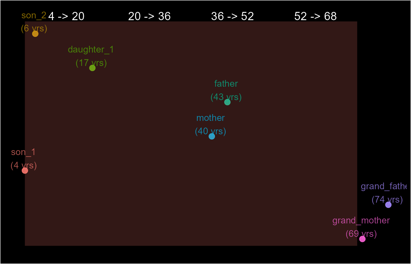
Despite the use of by and length.out, if
the configurations of records relative to the index record changes, the
resulting identifier can change as well. For example, if the
"mother" and "father" were five years younger,
this would place them in two different age gaps, resulting in a total of
four generations.
homes$alt_age <- homes$age
lgk <- homes$member %in% c("father", "mother")
homes$alt_age[lgk] <- homes$alt_age[lgk] - 5
homes$grp_4 <- partitions(homes$alt_age, by = 16,
                          separate = TRUE,
                          windows_total = number_line(3, 4))
homes
#>         member age     grp_1     grp_2    grp_3 alt_age    grp_4
#> 1        son_1   4 PN.08 (I) PN.08 (I) PN.1 (I)       4 PN.1 (I)
#> 2        son_2   6 PN.08 (D) PN.08 (D) PN.2 (I)       6 PN.2 (I)
#> 3   daughter_1  17 PN.09 (I) PN.08 (D) PN.3 (I)      17 PN.3 (I)
#> 4       father  43 PN.10 (D) PN.10 (D) PN.4 (I)      38 PN.4 (I)
#> 5       mother  40 PN.10 (I) PN.10 (I) PN.5 (I)      35 PN.5 (I)
#> 6 grand_father  74 PN.12 (D) PN.06 (I) PN.6 (I)      74 PN.6 (I)
#> 7 grand_mother  69 PN.12 (I) PN.07 (I) PN.7 (I)      69 PN.7 (I)

schema(homes$grp_4, seed = 4,
       custom_label = paste0(homes$member, " \n(", homes$alt_age, " yrs)"))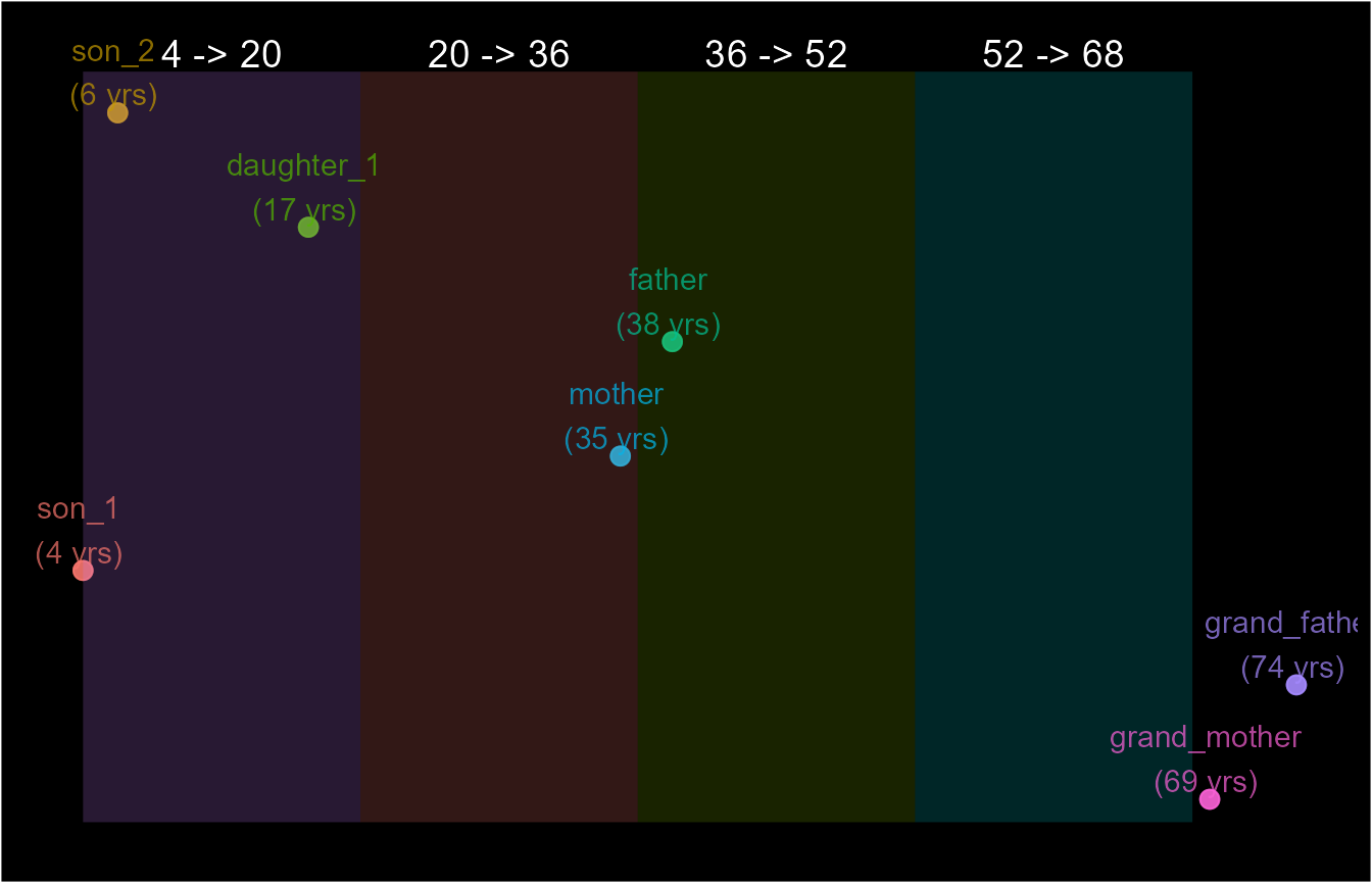
This makes a difference if our conditions changes to only three generations as the condition for our three-generation households.
homes$grp_5 <- partitions(homes$alt_age, by = 16,
                          separate = FALSE,
                          windows_total = number_line(3, 3))

homes
#>         member age     grp_1     grp_2    grp_3 alt_age    grp_4    grp_5
#> 1        son_1   4 PN.08 (I) PN.08 (I) PN.1 (I)       4 PN.1 (I) PN.1 (I)
#> 2        son_2   6 PN.08 (D) PN.08 (D) PN.2 (I)       6 PN.2 (I) PN.2 (I)
#> 3   daughter_1  17 PN.09 (I) PN.08 (D) PN.3 (I)      17 PN.3 (I) PN.3 (I)
#> 4       father  43 PN.10 (D) PN.10 (D) PN.4 (I)      38 PN.4 (I) PN.4 (I)
#> 5       mother  40 PN.10 (I) PN.10 (I) PN.5 (I)      35 PN.5 (I) PN.5 (I)
#> 6 grand_father  74 PN.12 (D) PN.06 (I) PN.6 (I)      74 PN.6 (I) PN.6 (I)
#> 7 grand_mother  69 PN.12 (I) PN.07 (I) PN.7 (I)      69 PN.7 (I) PN.7 (I)
schema(homes$grp_5, seed = 4,
       custom_label = paste0(homes$member, " \n(", homes$alt_age, " yrs)"))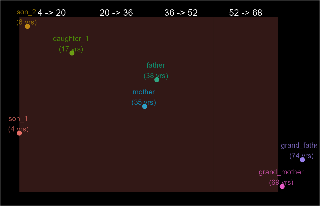
We see that the household no longer has a common identifier that
would identify it as a three-generation household. If we wish to address
this, then episodes() would be the better option.
homes$grp_6 <- episodes(homes$alt_age, case_length = 16)
homes
#>         member age     grp_1     grp_2    grp_3 alt_age    grp_4    grp_5
#> 1        son_1   4 PN.08 (I) PN.08 (I) PN.1 (I)       4 PN.1 (I) PN.1 (I)
#> 2        son_2   6 PN.08 (D) PN.08 (D) PN.2 (I)       6 PN.2 (I) PN.2 (I)
#> 3   daughter_1  17 PN.09 (I) PN.08 (D) PN.3 (I)      17 PN.3 (I) PN.3 (I)
#> 4       father  43 PN.10 (D) PN.10 (D) PN.4 (I)      38 PN.4 (I) PN.4 (I)
#> 5       mother  40 PN.10 (I) PN.10 (I) PN.5 (I)      35 PN.5 (I) PN.5 (I)
#> 6 grand_father  74 PN.12 (D) PN.06 (I) PN.6 (I)      74 PN.6 (I) PN.6 (I)
#> 7 grand_mother  69 PN.12 (I) PN.07 (I) PN.7 (I)      69 PN.7 (I) PN.7 (I)
#>              grp_6
#> 1  E.1 4 -> 17 (C)
#> 2  E.1 4 -> 17 (D)
#> 3  E.1 4 -> 17 (D)
#> 4 E.5 35 -> 38 (D)
#> 5 E.5 35 -> 38 (C)
#> 6 E.7 69 -> 74 (D)
#> 7 E.7 69 -> 74 (C)

schema(homes$grp_6, seed = 4,
       show_labels = c("length_arrow", "length"),
       custom_label = paste0(homes$member, " \n(", homes$alt_age, " yrs)"))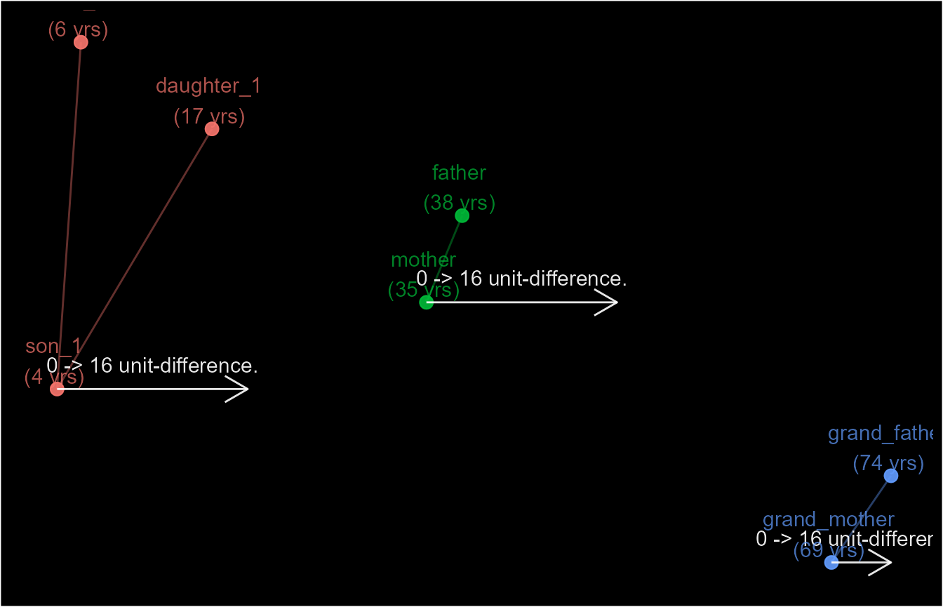
Unlike partitions(), additional analyses is required to
flag the whole household as a three-generation household. For example,
we can count the number of “occurrences” ( age gaps in epid
talk).
as.data.frame(homes$grp_6)
#>   epid sn     case_nm dist_wind_index dist_epid_index epid_length epid_total
#> 1    1  1        Case               0               0          13          3
#> 2    1  2 Duplicate_C               2               2          13          3
#> 3    1  3 Duplicate_C              13              13          13          3
#> 4    5  4 Duplicate_C               3               3           3          2
#> 5    5  5        Case               0               0           3          2
#> 6    7  6 Duplicate_C               5               5           5          2
#> 7    7  7        Case               0               0           5          2
#>   iteration wind_id1 wind_nm1 epid_start epid_end
#> 1         1        1     Case          4       17
#> 2         1        1     Case          4       17
#> 3         1        1     Case          4       17
#> 4         2        5     Case         35       38
#> 5         2        5     Case         35       38
#> 6         3        7     Case         69       74
#> 7         3        7     Case         69       74

homes$t3_home <- length(unique(homes$grp_6@wind_id[[1]])) == 3
homes
#>         member age     grp_1     grp_2    grp_3 alt_age    grp_4    grp_5
#> 1        son_1   4 PN.08 (I) PN.08 (I) PN.1 (I)       4 PN.1 (I) PN.1 (I)
#> 2        son_2   6 PN.08 (D) PN.08 (D) PN.2 (I)       6 PN.2 (I) PN.2 (I)
#> 3   daughter_1  17 PN.09 (I) PN.08 (D) PN.3 (I)      17 PN.3 (I) PN.3 (I)
#> 4       father  43 PN.10 (D) PN.10 (D) PN.4 (I)      38 PN.4 (I) PN.4 (I)
#> 5       mother  40 PN.10 (I) PN.10 (I) PN.5 (I)      35 PN.5 (I) PN.5 (I)
#> 6 grand_father  74 PN.12 (D) PN.06 (I) PN.6 (I)      74 PN.6 (I) PN.6 (I)
#> 7 grand_mother  69 PN.12 (I) PN.07 (I) PN.7 (I)      69 PN.7 (I) PN.7 (I)
#>              grp_6 t3_home
#> 1  E.1 4 -> 17 (C)    TRUE
#> 2  E.1 4 -> 17 (D)    TRUE
#> 3  E.1 4 -> 17 (D)    TRUE
#> 4 E.5 35 -> 38 (D)    TRUE
#> 5 E.5 35 -> 38 (C)    TRUE
#> 6 E.7 69 -> 74 (D)    TRUE
#> 7 E.7 69 -> 74 (C)    TRUE
Similar to episodes(), everything we’ve discussed above
can be done separately for different subsets of the dataset by using the
strata argument. For example, different households.
duplicate <- rbind(homes[1:2], homes[1:2])
duplicate$house_hold <- c(rep("london", 7), rep("hull", 7))

duplicate$grp_1 <- partitions(duplicate$age, by = 16,
                               separate = FALSE,
                               windows_total = number_line(3, 4),
                               strata = duplicate$house_hold)
duplicate$grp_2 <- episodes(duplicate$age,
                             case_length = 16,
                             strata = duplicate$house_hold)
duplicate
#>          member age house_hold     grp_1             grp_2
#> 1         son_1   4     london PN.01 (I)  E.01 4 -> 17 (C)
#> 2         son_2   6     london PN.02 (I)  E.01 4 -> 17 (D)
#> 3    daughter_1  17     london PN.03 (I)  E.01 4 -> 17 (D)
#> 4        father  43     london PN.04 (I) E.05 40 -> 43 (D)
#> 5        mother  40     london PN.05 (I) E.05 40 -> 43 (C)
#> 6  grand_father  74     london PN.06 (I) E.07 69 -> 74 (D)
#> 7  grand_mother  69     london PN.07 (I) E.07 69 -> 74 (C)
#> 8         son_1   4       hull PN.08 (I)  E.08 4 -> 17 (C)
#> 9         son_2   6       hull PN.09 (I)  E.08 4 -> 17 (D)
#> 10   daughter_1  17       hull PN.10 (I)  E.08 4 -> 17 (D)
#> 11       father  43       hull PN.11 (I) E.12 40 -> 43 (D)
#> 12       mother  40       hull PN.12 (I) E.12 40 -> 43 (C)
#> 13 grand_father  74       hull PN.13 (I) E.14 69 -> 74 (D)
#> 14 grand_mother  69       hull PN.14 (I) E.14 69 -> 74 (C)
schema(duplicate$grp_1, seed = 5,
       custom_label = paste0(duplicate$member, " (", duplicate$age, " yrs) in \n", duplicate$house_hold))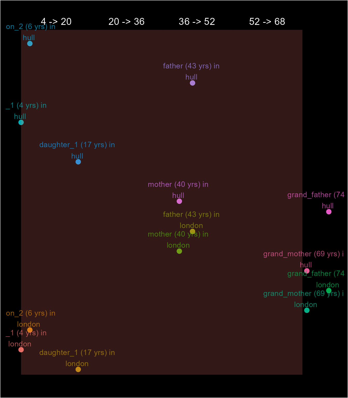
schema(duplicate$grp_2, seed = 4,
       show_labels = c("length_arrow", "length"),
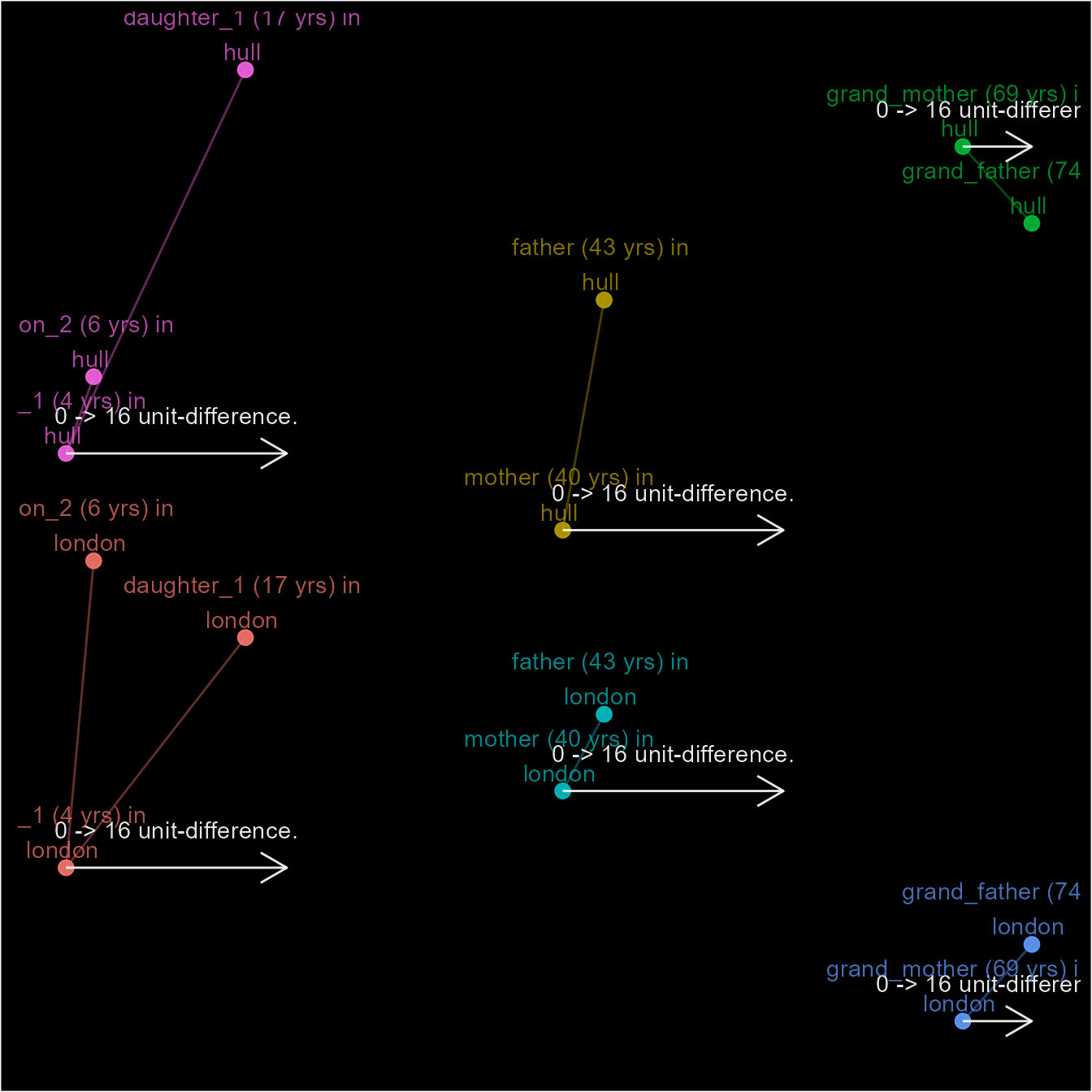
       custom_label = paste0(duplicate$member, " (", duplicate$age, " yrs) in \n", duplicate$house_hold))